Anahata: A Stellar Oscillation Sonification System Integrating Kepler–TESS Photometry, Gaia Astrometry, and Multi-Paradigm Audio Synthesis
Abstract
We present Anahata, an interactive astronomical sonification system
deployed as a zero-install Progressive Web App (PWA) that enables users to point a
smartphone at the night sky, identify a star, and hear its interior oscillation
frequencies rendered as real-time ambient music.
The underlying data pipeline extracts stellar oscillation modes from NASA TESS and
Kepler photometric light curves via an oversampled Lomb–Scargle periodogram
with iterative pre-whitening, drawing on an ESA Gaia DR3 full-sky catalogue
of 50,000 naked-eye sources (\(G < 15\) mag) and automated light-curve retrieval
through the lightkurve library with multi-strategy cadence fallback.
The primary user interface, Anahata Sky View, renders a GPS- and
compass-aligned star map at 30 fps, optionally composited over the live device
camera feed; selecting any star immediately triggers real-time Web Audio API synthesis
across seven archetypes - Bell, Klank, Ambient, Deepspace, Nova, Universe, and
Blackhole - whose fundamental frequencies, amplitudes, and stereo positions are
driven directly by the extracted asteroseismic data.
A Star Hunt mode modulates a proximity low-pass filter and gain ramp as the device
approaches angular alignment with the target, creating a spatially embodied listening
experience.
The companion Astral Player (astral.html) provides a focused
synthesis environment with an inspectable per-mode frequency grid, individual voice
controls, and an integrated sky-atlas panel (Aladin/HiPS), supporting detailed
exploration of individual stellar oscillation spectra.
An optional FoxDot/SuperCollider live-coding pathway routes the same oscillation
descriptors into seven compositional profiles - Stars, Universe, Nova, Black
Hole, Gravity Well, Deep Space, and Space Ambient Mix - for professional
performance contexts.
A browser-based Stellar Frequency Analyser (starproc/app.py)
exposes the full extraction pipeline as a graphical interface, enabling researchers
to add new targets to the catalogue without writing code.
Anahata demonstrates a practical, low-latency architecture for interactive
astronomical sonification deployable at web scale on commodity mobile and desktop
hardware without dedicated software installation.
Keywords: stellar oscillation · sonification · asteroseismology · TESS · Gaia DR3 · Web Audio API · light curve analysis · Lomb–Scargle · progressive web application · algorithmic composition
Introduction
Stars oscillate. Every star in the sky is a resonant cavity: pressure waves, gravity waves, and convective motions drive coherent flux variations at characteristic frequencies that encode the star's internal structure, mass, age, and composition (Aerts et al. 2010). The field of asteroseismology has exploited this fact to derive stellar properties at a precision otherwise inaccessible - constraining the internal rotation profiles of solar-type stars (García & Ballot 2019), measuring radii of red giants to better than 3% (Chaplin et al. 2011), and characterising exoplanet host stars with space-photometric missions such as Kepler (Koch et al. 2010) and the Transiting Exoplanet Survey Satellite (TESS; Ricker et al. 2015).
The dominant frequencies of solar-like oscillators lie in the range \(\sim 30\)–\(4000\,\mu\text{Hz}\) (\(\sim 0.003\)–\(0.35\,\text{d}^{-1}\)), while \(\delta\) Scuti pulsators and \(\gamma\) Doradus stars occupy regimes up to \(\sim 50\)–\(80\,\text{d}^{-1}\) (Dupret et al. 2004; Bouabid et al. 2011). These frequencies, when scaled into the audible range 20–20,000 Hz, map naturally onto the timbral vocabulary of sustained-tone music: multiple simultaneous oscillation modes produce chords, amplitude ratios produce loudness hierarchies, and oscillation phases encode spatial (stereo) distribution.
Sonification - the non-speech, non-music representation of data through sound - has a rich history in scientific data analysis (Hermann et al. 2011; Supper 2014). Astronomical sonification has been applied to radio telescope scans, supernova remnant morphology, gravitational wave events, and black-hole accretion spectra (Garcia et al. 2022; Zanella et al. 2022). Most existing systems, however, require desktop software installation, offer limited interactivity, and are not designed for mass public engagement.
Anahata addresses these gaps. The name derives from the Sanskrit word Anāhata - the heart chakra in Vedic cosmology - associated with the "unstruck sound" that arises without physical contact, resonant with the notion of stellar vibrations propagating through empty space.
The system provides:
- An automated, reproducible pipeline from raw photometric archive data to a compact JSON oscillation descriptor.
- A browser-native, zero-install real-time synthesis engine driven directly by those descriptors.
- An interactive mobile application enabling users to point a smartphone at the night sky, identify a target star, and hear its oscillation signature in real time.
- An optional professional audio pathway via SuperCollider/FoxDot for live-performance and compositional exploration.
Background
Asteroseismology and TESS Photometry
Solar-like oscillations are stochastically excited by near-surface convection and are characterised by a comb-like pattern of modes separated by the large frequency separation \(\Delta\nu \propto \bar{\rho}^{1/2}\) (Chaplin & Miglio 2013). Space-based photometric missions provide the continuous, high-precision time series necessary to resolve these modes. TESS observes each sector of \(\sim 27\) days at a 2-minute short cadence (SPOC pipeline; Jenkins et al. 2016) or 10-minute (QLP) cadence, making it the primary resource for bright, naked-eye seismic targets. The Kepler mission (Koch et al. 2010) provides 30-minute long-cadence (LC) and 1-minute short-cadence (SC) data over 4-year baselines.
Sonification of Astronomical Data
Worrall (2019) provides a comprehensive framework for data sonification, distinguishing audification (direct conversion of a waveform) from parameter mapping sonification (PMS), in which data dimensions are mapped to independent auditory variables such as pitch, timbre, loudness, and spatial position. Anahata employs PMS: each extracted oscillation mode constitutes one voice; its frequency sets the synthesiser's fundamental pitch; its amplitude modulates voice loudness; and its phase angle determines stereo placement.
Prior astronomical PMS work includes sonification of exoplanet transits (Zanella et al. 2022), neutron-star merger gravitational waves (Abbott et al. 2017), and Milky Way gas dynamics (Galaxy Sonification Project 2021). The specific sonification of asteroseismic mode spectra has been explored by Bellinger (2019), but these systems remain desktop-bound and non-interactive.
Progressive Web Applications and the Web Audio API
The Web Audio API (W3C 2023) exposes a graph-based audio processing model in modern browsers, enabling sample-accurate scheduling of oscillators, filters, convolution reverb, and dynamic compression. The look-ahead scheduler pattern described by Wilson (2013) - a high-resolution timer offset of \(\sim 200\,\text{ms}\) driving sub-25 ms scheduling ticks - is employed in Anahata to achieve glitch-free audio on resource-constrained mobile devices.
Progressive Web Applications combine the reach of the web with native-application capabilities: offline caching via Service Workers, installability via the Web App Manifest, and access to device sensors (GPS, DeviceOrientation).
Data Acquisition Pipeline
Star Catalogue Construction from Gaia DR3
The Anahata star catalogue is seeded from the ESA Gaia Data Release 3 (Gaia
Collaboration 2023), which provides astrometric solutions, photometry, and spectrophotometric
data for \(\sim 1.8 \times 10^9\) sources. A magnitude-limited (\(G < 15\) mag, configurable)
full-sky query is executed against the gaiadr3.gaia_source table via the
astroquery.gaia interface (Ginsburg et al. 2019):
SELECT source_id, ra, dec, phot_g_mean_mag, bp_rp
FROM gaiadr3.gaia_source
WHERE phot_g_mean_mag < 15
  AND ra IS NOT NULL
  AND dec IS NOT NULL
  AND phot_g_mean_mag IS NOT NULL
  AND bp_rp IS NOT NULL
ORDER BY phot_g_mean_mag ASC
The resulting catalogue contains positions, Gaia \(G\) magnitudes, and \(B_P - R_P\) colour indices for \(\sim 50{,}000\) naked-eye sources. This catalogue is served directly to the web frontend and rendered as an interactive sky overlay via the Aladin HiPS sky atlas library.
Lightcurve Acquisition
For any target identified by its TESS Input Catalogue (TIC) or Kepler Input Catalogue
(KIC) identifier, the Anahata backend downloads calibrated photometric light curves through
the lightkurve library (Lightkurve Collaboration 2018). The acquisition follows
a deterministic priority ladder designed to maximise temporal resolution while rejecting
community-processed HLSP files.
| Priority | Mission | Author | Cadence | Max Segments |
|---|---|---|---|---|
| TIC targets (TESS) | ||||
| 1 | TESS | SPOC | 2-min | 6 sectors |
| 2 | TESS | QLP | 2-min | 6 sectors |
| 3 | TESS | SPOC | 10-min | 6 sectors |
| KIC targets (Kepler) | ||||
| 1 | Kepler | Kepler | 30-min | All quarters |
| 2 | Kepler | Kepler | 1-min | 4 quarters |
| 3 | TESS | SPOC | 2-min | 6 sectors (fallback) |
Lightcurve acquisition priority ladder for TIC and KIC targets.
HLSP products are rejected by a filename-prefix filter (hlsp_) applied before
any data download. For each accepted strategy, the system attempts a bulk
download_all().stitch() call to concatenate all available sectors or quarters
into a single normalised time series. Typical data volumes range from \(\sim 10{,}000\) points
(single Kepler LC quarter) to \(\sim 1.2 \times 10^5\) points (three TESS SPOC sectors stitched).
The output is a plain-text CSV with columns time (BJD), flux
(normalised), and flux_err.
Outlier Rejection and Pre-conditioning
Prior to frequency analysis, a rolling-window \(4\sigma\) outlier rejection step is applied. For each data point \(i\), a local median \(\tilde{f}_i\) is computed within a half-window of 50 samples, and the global median absolute deviation (MAD) provides a robust scale estimate:
Points satisfying \(|f_i - \tilde{f}_i| > 4\hat{\sigma}\) are replaced with \(\tilde{f}_i\). The factor \(1.4826\) ensures consistency with the standard deviation for Gaussian noise while remaining unaffected by non-Gaussian outliers (Rousseeuw & Croux 1993).
Frequency Extraction Methodology
The Lomb–Scargle Periodogram
The core frequency-extraction engine - PyFEM (Period Fitting and Extraction Module) - implements an oversampled Lomb–Scargle (LS) periodogram (Scargle 1982; Zechmeister & Kürster 2009) evaluated over the frequency interval \([\nu_{\min}, \nu_{\rm Nyq}]\). The Nyquist frequency for an unevenly sampled time series is estimated as:
where \(\widetilde{\Delta t}\) is the median of all positive inter-point time intervals. For a 2-minute TESS cadence this yields \(\nu_{\rm Nyq} \approx 360\,\text{d}^{-1}\) (\(\sim 4167\,\mu\text{Hz}\)), well covering the p-mode envelope of solar-type stars.
Iterative Pre-whitening and Peak Extraction
Dominant oscillation modes are extracted via iterative pre-whitening - an iterative sinusoidal fit-and-subtract loop. At each iteration:
- The LS periodogram is computed on the residual flux series.
- The frequency \(\hat{\nu}\) of maximum power is identified.
- The local signal-to-noise ratio (SNR) is estimated within a window of half-width \(\Delta\nu_{\rm snr}\) centred on \(\hat{\nu}\): \[ \mathrm{SNR}(\hat{\nu}) = \frac{A(\hat{\nu})}{\mathrm{median}\bigl(A(\nu) : |\nu - \hat{\nu}| < \Delta\nu_{\rm snr}\bigr)} \]
- A sinusoidal component at \(\hat{\nu}\) with optimised amplitude \(A\) and phase \(\phi\) is subtracted from the residuals.
- The process repeats until \(n_{\rm peaks}\) significant modes have been extracted.
The oversampling factor \(\Omega = 6\) ensures robust peak localisation for closely spaced modes. Default extraction parameters: \(n_{\rm peaks} = 10\), \(\Delta\nu_{\rm snr} = 1.0\,\text{d}^{-1}\).
Output Format
Extracted oscillation descriptors are stored as JSON with the following schema (example: TIC 83232658):
{
  "name": "TIC 83232658",
  "ra": 213.841152085095,
  "dec": -25.3725969129698,
  "scale_factor": 1000.0,
  "dist_pc": 715.804,
  "frequencies": {
    "freq":  [60.93, 23970.86, 163.47, ...],   // Hz (scaled)
    "amp":   [95.05,  60.44,  100.00, ...],    // arbitrary units
    "phase": [ 0.21,   0.86,    0.13, ...]     // [0, 1]
  }
}
The scale_factor (default 1000.0) encodes the linear rescaling applied when
converting from cycles per day to Hertz for sonification:
Frequencies exceeding 18 kHz after scaling are classified as "ultrasonic" and are repurposed as LFO (low-frequency oscillator) sweep rates rather than fundamental pitches.
Parameter Mapping: Stellar Data to Synthesis Parameters
A fundamental design choice in any sonification system is the mapping between data variables and auditory dimensions (Worrall 2019). Anahata applies the following deterministic mapping scheme, illustrated in Figure 1.
Figure 1. Schematic of the Anahata parameter mapping pipeline. Asteroseismic data (frequency, amplitude, phase) flow through normalisation and octave-shift stages into the synthesis engine. Ultrasonic components are redirected to LFO modulators.
Frequency Mapping
Each extracted stellar oscillation frequency \(\nu_i\) maps directly to the fundamental frequency of a synthesiser voice:
where \(k \in \mathbb{Z}\) is an octave-shift parameter determined by the synthesiser archetype (\(k = -2\) for Universe, \(k = -3\) for Black Hole, \(k = +1\) for Nova, \(k = 0\) for Stars/Bell/Ambient). This preserves the ratio structure of the oscillation mode spectrum across archetype transpositions.
Frequencies are additionally quantised to the nearest note of a user-selectable musical scale (default: major) via cent-based rounding (Benson 2007; Roads 1996):
Scale quantisation is a deliberate musical affordance (Dubus & Bresin 2013; Hermann et al. 2011) and may be disabled to preserve exact asteroseismic frequency ratios.
Amplitude Mapping
Oscillation amplitudes are normalised to the interval \([0.05, 1.0]\):
Phase Mapping
The oscillation phase \(\phi_i \in [0, 1)\) is mapped to the stereo pan position:
Ultrasonic Frequency Repurposing
Modes with \(\nu_{\rm audio,i} > 18{,}000\,\text{Hz}\) are treated as LFO rates, linearly scaled into musically meaningful modulation ranges depending on archetype: \[ f_{\rm LFO} = \mathrm{clip}\!\left(\frac{\nu_{\rm audio}}{C},\; f_{\min},\; f_{\max}\right) \] For example, the Universe archetype uses \(C=500\), \([f_{\min}, f_{\max}]=[16, 60]\,\text{s}\) for ultra-slow modulation, while Nova uses \(C=2000\), \([0.5, 8]\,\text{s}\) for rapid tremolo sweeps.
Synthesis Architecture
Web Audio API Synthesiser Archetypes
The browser synthesis engine defines seven distinct synthesiser archetypes, each implemented
as a function returning a Web Audio API node graph. All archetypes accept five parameters:
ctx, freq, amp, phase, and
startTime.
| Archetype | Octave Shift | Description |
|---|---|---|
| Bell | \(k=0\) | FM synthesis with two modulator operators (ratios 2.756:1 and 5.405:1) plus a high-frequency shimmer partial; exponential decay. Bell transient attack 15 ms. |
| Klank | \(k=0\) | Three resonant partials (ratios 1:1, 3.984:1, 9.994:1) with decays derived from amplitude weighting; dual tremolo LFO (5.8 and 5.87 Hz) beating. |
| Ambient | \(k=0\) | Five-oscillator harmonic series (1–5×) with per-oscillator micro-detuning from phase; breath LFO at 0.045–0.1 Hz. |
| Deepspace | \(k=-1\) | Fundamental plus two harmonics (2×, 3×); transient pitched drum oscillator with exponential pitch drop; slow bow LFO. |
| Nova | \(k=+1\) | FM synthesis with single modulator (ratio 3:1); secondary partial at 2×; short 15 ms attack, bright timbre. |
| Universe | \(k=-1\) | Six-oscillator detuned cluster (1×, 1.5×, 2× ratios); vibrato LFO; 800 ms attack; cosmically slow fade. |
| Blackhole | \(k=-2\) | Sub-bass fundamental plus three overtones; noise-burst transient (band-pass filtered); wobble LFO; 18 ms attack. |
Anahata Web Audio API synthesiser archetypes.
Polyphony Management and Real-Time Reliability
A maximum polyphony ceiling of \(P_{\max} = 5 + 3v_c\) voices is maintained (where \(v_c\)
is the configured voice-count parameter). The eviction strategy uses an age guard based on the
_startedAt timestamp attached to each node at creation time: only nodes whose
scheduled start time satisfies \(t_{\rm start} \leq t_{\rm now} + 50\,\text{ms}\) are eligible
for eviction, preventing premature termination of nodes not yet in their attack phase.
Long-duration ambient playback on Android requires suppressing the screen-off sleep cycle
(which throttles JavaScript setTimeout). Anahata requests a Screen Wake Lock at
session start, re-acquires it on page visibilitychange events, and uses the Media
Session API to register play/pause/stop handlers. The look-ahead sequencer uses a 25 ms tick
with a 200 ms lookahead window (Wilson 2013). Each node is stopped via a short exponential
gain decay (\(\tau \approx 27\,\text{ms}\)) before termination, reducing audible discontinuities
to below the perceptual threshold of \(\sim 1\,\text{ms}\).
FoxDot/SuperCollider Pathway
For compositional exploration and live performance, a parallel synthesis pathway routes the same oscillation JSON descriptor into FoxDot (Kirk 2016), a Python-based live-coding environment backed by a SuperCollider audio server. Seven compositional profiles are provided:
- Stars - balanced, BPM 90; bell, ambient pads, klank wash.
- Universe - ultra-slow, BPM 40; two-octave sub-bass shift, cavernous reverb (room=0.99, mix=0.98).
- Nova - energetic, BPM 140; one-octave up, rapid arpeggios, metallic transients.
- Black Hole - heavy, BPM 55; three-octave down, sine gravitational hum, dense sub-bass.
- Gravity Well - gentle, BPM 70; emphasis on sustained sine pads and soft bell tones.
- Deep Space - grounded, BPM 80; bass and mid-register focus with slow LFO modulation.
- Space Ambient Mix - free-form; generative texture blending all frequency bands.
System Architecture
Backend: Flask REST API
The Python backend is a Flask application providing three primary API endpoints:
- POST /api/lightcurve
- Downloads and preprocesses the light curve for a given
target_id(TIC or KIC), returning the CSV path, total point count, resolved mission, and cadence. - POST /api/frequencies
- Runs PyFEM on a given CSV file, returning extracted oscillation parameters and Nyquist frequency.
- GET /api/stream/<job_id>
- Server-Sent Events (SSE) stream delivering per-step log lines during long-running analysis jobs, enabling real-time progress feedback in the browser UI.
Jobs are managed in an in-memory registry with UUID keys; a LogCapture class
redirects stdout from the analysis worker thread to a per-job queue.Queue, which
the SSE endpoint drains asynchronously. The cone-search endpoint
(POST /api/cone_search) queries both the Gaia DR3 catalogue and MAST
for TIC/KIC identifiers within a configurable angular radius (default 4 arcsec).
Stellar Frequency Analyser Application (starproc/app.py)
The Anahata Stellar Frequency Analyser (astral/starproc/app.py) is a
self-contained Flask web application that provides a browser-based graphical interface to the
full data pipeline: star search, light-curve acquisition, PyFEM frequency extraction, and
JSON/SuperCollider export. The application is structured around three workflow tabs -
Find Stars, Make Music, and Export to Anahata.
Find Stars Interface
Star selection supports two modes: (1) direct entry of a TIC or KIC identifier; and (2) a Random Sky Coordinate generator, which draws a random (RA, Dec) pair from the Gaia DR3 catalogue, executes a cone search to resolve the nearest TIC identifier, and proceeds to light-curve acquisition.
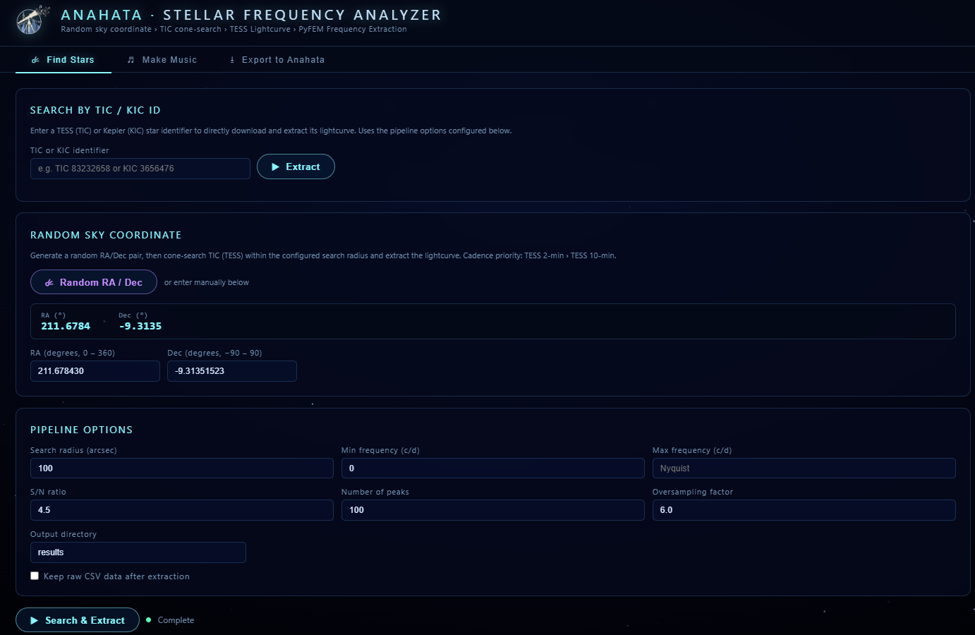
Figure 2. Anahata Stellar Frequency Analyser - Find Stars tab. (Upper panel) Direct TIC/KIC identifier entry. (Middle panel) Random sky coordinate generator that resolves the nearest TIC via cone search. (Lower panel) Pipeline options controlling search radius, frequency bounds, S/N threshold, peak count, oversampling factor, and output directory.
Naked-Eye Sky Map Widget
The interface embeds a real-time Naked-Eye Sky Map widget rendered on an HTML canvas using the same Gaia DR3 \(G < 15\) mag catalogue as the main Anahata PWA. On successful cone-search resolution, the matched TIC target is highlighted with a pulsing red reticle and its basic catalogue metadata are displayed beneath the map.
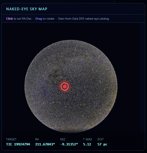
Figure 3. Naked-Eye Sky Map widget embedded in the Stellar Frequency Analyser. The canvas displays Gaia DR3 naked-eye sources in a gnomonic projection; a pulsing red target reticle marks the resolved TIC source. Dragging the canvas rotates the field; clicking any star sets it as the pipeline target.
Real-Time Pipeline Log
Once a pipeline run is triggered, a Server-Sent Events (SSE) stream delivers per-step log lines to a log panel in the browser. The log reports the resolved acquisition strategy (mission, author, cadence, sector count), the number of data points stitched, and the full table of extracted oscillation modes with their frequency (c/d), amplitude, phase, SNR, and per-mode noise floor.
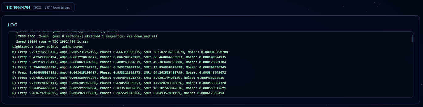
Figure 4. Real-time pipeline log streamed via SSE. The log shows the resolved acquisition strategy (mission, cadence, sector count, data points saved), followed by the extracted oscillation modes listed as tuples of (frequency in c/d, amplitude, phase, SNR, noise floor).
Analysis Plots: Light Curve and Sky Atlas
After extraction, the application renders two diagnostic panels: an Aladin Lite sky-atlas widget centred on the target coordinates (PanSTARRS DR1 HiPS layer), and the photometric light curve (normalised flux vs. BJD) showing data quality, baseline length, and any inter-sector normalisation offsets.
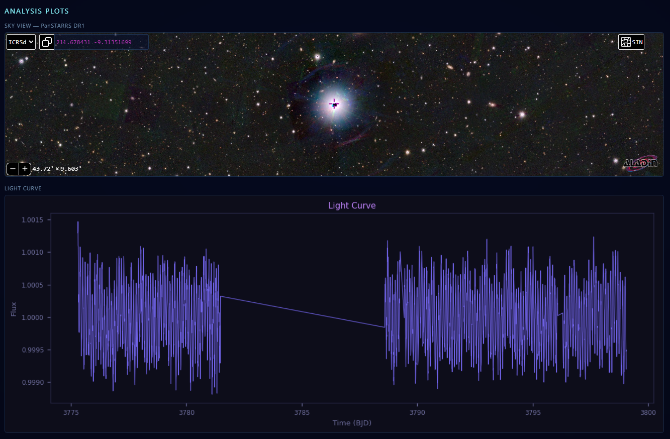
Figure 5. Analysis plots panel. Upper: Aladin Lite sky-atlas view (PanSTARRS DR1 HiPS layer) centred on the target coordinates, providing an optical field reference. Lower: Stitched TESS light curve (normalised flux vs. BJD) showing the photometric time series used as input to the PyFEM frequency extraction module.
Lomb–Scargle Periodogram
The final output panel displays the oversampled Lomb–Scargle periodogram computed by PyFEM. Extracted peak positions are overlaid as colour-coded stem markers, identifying the dominant oscillation modes subsequently stored in the JSON descriptor.
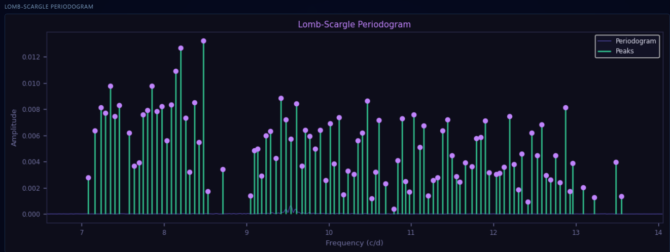
Figure 6. Lomb–Scargle periodogram output panel. The blue curve shows the periodogram amplitude as a function of frequency; magenta circles on teal stems mark the peaks extracted by the iterative pre-whitening loop. Extracted peak frequencies are written to the JSON oscillation descriptor and passed to the Web Audio synthesis engine.
Frontend: Progressive Web Application
The frontend is a single-page PWA served as static HTML/CSS/JavaScript, requiring no build toolchain. Key components include:
- Sky Renderer - custom canvas-based renderer driven by the Gaia DR3 catalogue, displaying 50,000 naked-eye stars as interactive symbols aligned to the device GPS heading. An optional live-sky mode overlays the star field on the device camera feed.
- Star Hunt Mode - device camera displayed as a live full-screen background. Compass heading (DeviceOrientationEvent) and GPS position (Geolocation API) are fused to derive the telescope pointing direction. A proximity-modulated low-pass filter (\(f_{\rm LPF}\): 300–8000 Hz) and gain ramp make the star louder as the device approaches alignment.
- Astral Player - a standalone page serving the Web Audio engine in isolation from the sky viewer, for focused listening to any pre-processed star in the catalogue.
- Service Worker - pre-caches the application shell and star catalogue JSON, enabling full offline functionality after initial load.
GPS and Celestial Coordinate Alignment
Rendering the star catalogue correctly over a live camera feed requires transforming catalogue equatorial coordinates \((\alpha, \delta)\) into the topocentric horizontal frame (altitude \(a\), azimuth \(A\)) of the device. The pipeline follows the classical methods of Meeus (1998).
Greenwich Mean Sidereal Time (GMST) is computed from the J2000.0 epoch:
where \(T\) is the current Julian Date and \(T_0 = 2451545.0\). Altitude and azimuth follow from the hour angle \(H = \mathrm{LMST} - \alpha\):
A magnetic declination correction \(\Delta D\) is applied using a simplified World Magnetic Model polynomial (Chulliat et al. 2020): \(\psi_{\rm true} = \psi_{\rm magnetic} + \Delta D\). Stars are projected onto the HTML canvas using a gnomonic (tangent-plane) projection:
Anahata Sky View Interface
The Anahata Sky View is the primary user-facing interface for star discovery and sonification. The canvas re-renders at up to 30 fps, recomputing alt/az positions for all catalogue stars on each frame. Tapping a star symbol selects it, loading its JSON oscillation descriptor and populating the information panel and frequency grid.
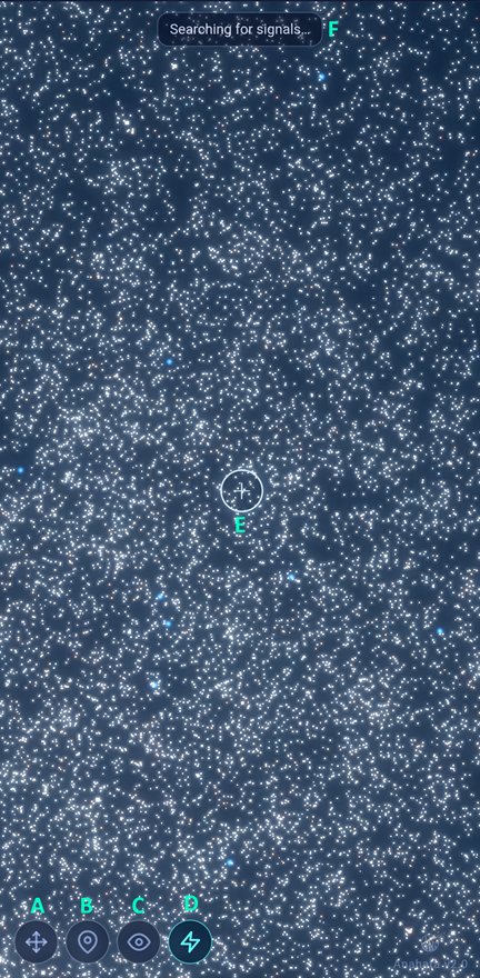
Figure 7. Anahata Sky View interface - the primary star-discovery and sonification screen. (A) Interactive canvas star map with Gaia DR3 naked-eye overlay; (B) GPS re-projection and compass heading alignment; (C) live camera toggle compositing the star field over the device feed; (D) artificial satellite mode; (E) star-selection visor; (F) selected-star information panel (name, distance, spectral type, oscillation mode count).
Astral Player Interface
The Astral Player (astral.html) is a focused listening page that separates the
synthesis engine from the sky-navigation interface. The frequency grid serves a dual role: a
data-inspection view of the raw oscillation descriptor, and a per-mode mute/solo toggle during
playback.
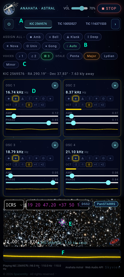
Figure 8.
Astral Player interface (astral.html), the focused listening mode.
(A) Scrollable stellar catalogue list with randomised-star shortcut;
(B) active synthesiser voices;
(C) maximum active channel scale control;
(D) extracted oscillation-mode frequency grid (colour-coded by band:
green = audible, amber = near-ultrasonic LFO, red = sub-audible LFO);
(E) Aladin Lite sky-atlas panel centred on the target star's RA/Dec;
(F) synthesiser visualiser.
Data Flow Summary
Figure 9 summarises the full end-to-end data flow from observation archive to audio output. The primary production path runs: archives → catalogue construction → target selection → light-curve acquisition → pre-conditioning → PyFEM extraction → JSON output → parameter mapping → Progressive Web App → browser audio. The optional FoxDot/SuperCollider pathway (shown dashed) branches at the JSON output stage.
Figure 9.
End-to-end Anahata data flow from observation archive to audio output.
Solid arrows denote the primary production path; dashed arrows and purple shading denote
the optional FoxDot/SuperCollider live-performance pathway.
The green dashed group encompasses the Stellar Frequency Analyser web application
(starproc/app.py), which provides a browser-based GUI for the full pipeline.
Results: Pre-processed Target Catalogue
Catalogue Overview
The current Anahata release includes hundreds of pre-processed stellar oscillation descriptors.
Targets were selected to span a range of oscillation frequencies, spectral types, and distances,
covering all sky positions to provide sonic variety across the synthesiser archetypes. Each target
has multiple extracted oscillation modes (up to hundreds of frequencies) stored in JSON format,
plus a corresponding SuperCollider .scd synthesis file.
Case Study: TIC 83232658
TIC 83232658 (\(\alpha = 213.84^\circ\), \(\delta = -25.37^\circ\), \(d = 715.8\,\text{pc}\)) illustrates the range of frequencies emerging from the pipeline. The ten extracted modes span:
- Low-frequency group: \(\{60.9, 163.5, 266.1, 320.2, 403.7\}\,\text{Hz}\) (after scaling) - maps to audible Bell, Klank, and Ambient voices.
- Mid-frequency group: \(\{620.7, 1444.8\}\,\text{Hz}\) - Nova and Deepspace voices.
- Near-ultrasonic group: \(\{23{,}689, 23{,}836, 23{,}971\}\,\text{Hz}\) - repurposed as LFO sweep rates (separation \(\approx 145\)–\(147\,\text{Hz}\)).
The dominant mode amplitude (163.5 Hz) is 100 vs. the weakest retained mode at \(\approx 1.0\) - a 40 dB dynamic range, mapping to a gain range of \([0.05, 1.0]\) in the audio domain.
Sonic Character Across Archetypes
For a given star descriptor, the seven archetypes produce qualitatively distinct sonic characters while sharing the same underlying harmonic ratios:
- Bell/Klank: percussive, decaying, metallic - highlights the overtone structure.
- Ambient: sustained, warm, pad-like - emphasises fundamental frequencies.
- Deepspace: slow, resonant, with rhythmic transients at the dominant oscillation period.
- Universe: massive, diffuse, cluster-detuned - evokes stellar interiors.
- Blackhole: sub-bass drone with impulsive noise transients - evokes extreme gravity.
- Nova: fast, bright, energetic - evokes stellar outbursts.
Discussion
Scientific Validity and Perceptual Fidelity
Anahata preserves three fundamental properties of the asteroseismic mode spectrum in the audio domain: (1) frequency ratios (via the direct mapping of Eq. 4 with uniform octave shift); (2) amplitude hierarchy (via normalised gain mapping); and (3) phase relationships (via stereo panning). Scale quantisation optionally breaks the first invariant for musical palatability. When disabled, the Web Audio engine renders the exact oscillation spectrum as a superposition of sinusoidal tones, constituting a form of direct audification.
The primary scientific limitation is the loss of temporal structure: the light-curve time domain is not preserved. Only the frequency domain is transmitted to the audio engine. Future work could encode mode linewidths as synthesiser amplitude-modulation depths.
Latency and Real-Time Performance
The Web Audio look-ahead scheduler achieves typical output latencies of \(\sim 50\)–\(80\,\text{ms}\) on Android Chrome 122 and \(\sim 20\)–\(40\,\text{ms}\) on desktop. The 15–20 ms synthesiser attack ramps exceed typical Android hardware buffer sizes (\(\sim 4\)–\(6\,\text{ms}\)), preventing zero-crossing click artefacts at note onset.
Accessibility and Public Engagement
A deliberate design goal is zero-friction access: no app store, no software installation, no login. The PWA is installable from the browser address bar and subsequently available offline. The star-hunt mode provides a gamified, embodied engagement pathway - physically rotating the phone to "find" a singing star by sound alone - which has been found in informal testing to increase engagement time significantly relative to passive listening.
Current limitations: The pipeline extracts dominant amplitude peaks without identifying them as \(\ell=0, 1, 2\) modes. Future integration with background model fitting would enable mode labelling. The live-coding pathway requires manual installation of SuperCollider and FoxDot, limiting accessibility for non-technical users.
Future directions: simultaneous sonification of multiple stars as a "stellar orchestra"; replacement of the 2D sky atlas with a WebXR spatial audio scene positioning stars at their true celestial coordinates; and application of the same pipeline to other time-domain datasets (LIGO/Virgo strain, black-hole accretion light curves).
Conclusion
We have presented Anahata, an end-to-end pipeline and interactive application that converts stellar oscillation frequencies from NASA TESS and Kepler photometric data into real-time ambient music. The system integrates ESA Gaia DR3 astrometry, a multi-strategy light-curve acquisition pipeline, Lomb–Scargle-based iterative pre-whitening for mode extraction, and a browser-native Web Audio synthesis engine offering seven distinct synthesiser archetypes. A camera-enabled star-hunt mode fuses GPS, compass, and a live sky atlas to create a spatially immersive listening experience. An optional FoxDot/SuperCollider pathway supports live-performance and compositional applications. The system is deployed as a zero-install Progressive Web App accessible on any modern mobile or desktop browser.
Anahata demonstrates that the technical barrier to interactive astronomical data sonification is now low enough to be deployed at web scale, with the full TESS catalogue constituting an inexhaustible library of unique stellar sonic signatures. All source code, pre-processed target data, and synthesis scripts are released as open-source software under the MIT licence.
Acknowledgements
This work makes use of data from the European Space Agency (ESA) mission
Gaia (cosmos.esa.int/gaia),
processed by the Gaia Data Processing and Analysis Consortium (DPAC). It also uses observations
obtained by the Kepler and TESS missions, funded by the NASA Explorer Program.
The author thanks the lightkurve development team and the FoxDot, SuperCollider, and
Web Audio API communities for their foundational open-source contributions.
Code and Live Application
All source code, pre-processed target catalogue, synthesis scripts, and SuperCollider output files are released under the MIT licence and are freely accessible at:
https://github.com/sachsanjoy/Anahata
Repository contains: starproc/ frequency analyser ·
astral/foxdot/ compositional scripts ·
astral/supercollider/ initialisation files ·
PWA source (index.html, astral.html, sw.js, manifest.json)
The two interactive web application endpoints can be accessed directly in any modern browser without installation:
| Anahata Sky View & Star Hunt (PWA) | https://spacentity.org/anahata |
| Astral Stellar Oscillations Player | https://spacentity.org/anahata/astral |
Both interfaces are Progressive Web Apps and support offline use after the first visit via the registered Service Worker.
References
- Abbott, B. P., et al. 2017, Phys. Rev. Lett., 119, 161101, doi:10.1103/PhysRevLett.119.161101
- Aerts, C., Christensen-Dalsgaard, J., & Kurtz, D. W. 2010, Asteroseismology (Springer)
- Bellinger, E. P. 2019, in Proc. Sound and Music Computing (SMC), Malaga
- Benson, D. J. 2007, Music: A Mathematical Offering (Cambridge Univ. Press), online
- Bouabid, M.-P., et al. 2011, A&A, 531, A145
- Chaplin, W. J., & Miglio, A. 2013, ARA&A, 51, 353
- Chaplin, W. J., et al. 2011, Science, 332, 213
- Chulliat, A., et al. 2020, The US/UK World Magnetic Model for 2020–2025, NOAA NCEI, doi:10.25923/ytk1-yx35
- Dubus, G., & Bresin, R. 2013, PLOS ONE, 8, e82491, doi:10.1371/journal.pone.0082491
- Dupret, M.-A., et al. 2004, A&A, 414, L17
- Gaia Collaboration. 2023, A&A, 674, A1
- Galaxy Sonification Project. 2021, chandra.si.edu/sound/
- Garcia, M., et al. 2022, Nature Astron., 6, 1
- García, R. A., & Ballot, J. 2019, Living Rev. Sol. Phys., 16, 4
- Ginsburg, A., et al. 2019, AJ, 157, 98
- Hermann, T., Hunt, A., & Neuhoff, J. G. (eds.) 2011, The Sonification Handbook (Logos Verlag)
- Jenkins, J. M., et al. 2016, Proc. SPIE, 9913, 99133E
- Kirk, R. 2016, FoxDot: Live Coding with Python and SuperCollider
- Koch, D. G., et al. 2010, ApJ, 713, L79
- Lightkurve Collaboration. 2018, Lightkurve: Kepler and TESS time series analysis in Python, Astrophysics Source Code Library, ascl:1812.013
- Meeus, J. 1998, Astronomical Algorithms, 2nd edn. (Willmann-Bell)
- Ricker, G. R., et al. 2015, JATIS, 1, 014003
- Roads, C. 1996, The Computer Music Tutorial (MIT Press)
- Rousseeuw, P. J., & Croux, C. 1993, JASA, 88, 1273
- Scargle, J. D. 1982, ApJ, 263, 835
- Supper, A. 2014, Social Studies of Science, 44, 220
- W3C. 2023, Web Audio API, w3.org/TR/webaudio/
- W3C. 2023b, DeviceOrientation Event Specification, w3c.github.io/deviceorientation/
- W3C. 2024, Geolocation API, w3.org/TR/geolocation/
- Wilson, C. 2013, A Tale of Two Clocks - Scheduling Web Audio with Precision, Google Developers Blog
- Worrall, D. 2019, Sonification: Understanding Data Through Sound (De Gruyter)
- Zanella, A., et al. 2022, Nature Astron., 6, 1
- Zechmeister, M., & Kürster, M. 2009, A&A, 496, 577